Spatial Randomforest
How to Run a RF Model
Although Random forest is a very powerful tool, it can be run fairly simply in R
#Lets read our libraries in first then load our shape file
library(rgdal)
library(raster)
library(sp)
library(randomForest)
library(tidyverse)

#We are going to extract points from a raster to a shapefile

WorkWD <- "C:/Users/User/Documents/R/Projects/R_Intro"

Training <- readOGR(dsn = WorkWD, layer = "TrainingData")
## OGR data source with driver: ESRI Shapefile
## Source: "C:\Users\User\Documents\R\Projects\R_Intro", layer: "TrainingData"
## with 100 features
## It has 5 fields
## Integer64 fields read as strings: OBJECTIDplot(Training)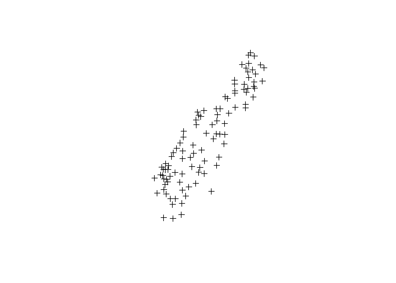
Coordinate Reference System and Spatial Projection
R is very picky about how we project our data, along with the geographical projection
#Apply a consitent CRS- Coordinate Reference System
proj4string(Training) <- CRS("+init=epsg:28992")
## Warning in showSRID(uprojargs, format = "PROJ", multiline = "NO", prefer_proj =
## prefer_proj): Discarded datum Amersfoort in Proj4 definition## Warning in proj4string(obj): CRS object has comment, which is lost in output## Warning in `proj4string<-`(`*tmp*`, value = new("CRS", projargs = "+proj=sterea +lat_0=52.1561605555556 +lon_0=5.38763888888889 +k=0.9999079 +x_0=155000 +y_0=463000 +ellps=bessel +units=m +no_defs")): A new CRS was assigned to an object with an existing CRS:
## +proj=stere +lat_0=90 +lat_ts=52.1561605555556 +lon_0=5.38763888888889 +x_0=155000 +y_0=463000 +ellps=bessel +units=m +no_defs
## without reprojecting.
## For reprojection, use function spTransform#The geographic projection has to be changed as well
Training <- spTransform(Training , CRS("+init=epsg:28992"))## Warning in showSRID(uprojargs, format = "PROJ", multiline = "NO", prefer_proj =
## prefer_proj): Discarded datum Amersfoort in Proj4 definitionRaster Data
Lets load in our raster data and see what it looks like.
#Load in the DEM and extract elevation values

#LOADINING THE RASTERS
DEM <- raster( file.path(WorkWD, "Elevationlow.tif"))
River <- raster(file.path(WorkWD, "Distance.tif"))

#lets plot the DEM to see what we have

plot(DEM)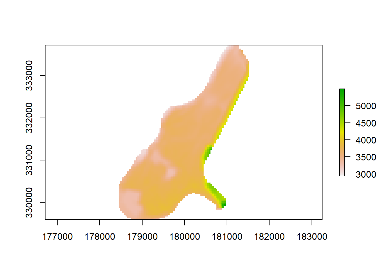
#Apply a consitent CRS
proj4string(DEM)<- CRS("+init=epsg:28992")
## Warning in showSRID(uprojargs, format = "PROJ", multiline = "NO", prefer_proj =
## prefer_proj): Discarded datum Amersfoort in Proj4 definitionproj4string(River)<- CRS("+init=epsg:28992")## Warning in showSRID(uprojargs, format = "PROJ", multiline = "NO", prefer_proj =
## prefer_proj): Discarded datum Amersfoort in Proj4 definition#Crop the River Raster to fit the DEM
#
River <- crop(River,DEM)Raster conversion and extract:
We can compute the slope and aspect as well The final function is the extract function, similar to the “extract multi values” tool in ArcGIS
#We are also creating a slope and aspect layer
Slope <- terrain(DEM, opt="slope", unit="degrees", neighbors=8)
Aspect <- terrain(DEM, opt="aspect", unit="degrees", neighbors=8)


#Extract Elevation Values
#raster::extract is saying to use the extract function directly from our raster package
Training$DEM <- raster::extract(DEM, Training, method = "simple")
Training$Slope <- raster::extract(Slope, Training, method = "simple")
Training$Aspect <- raster::extract(Aspect, Training, method = "simple")
Training$River <- raster::extract(River, Training, method = "simple")

#Lets check to see the summary statistics of our newly extracted data
summary(Training)
## Object of class SpatialPointsDataFrame
## Coordinates:
## min max
## coords.x1 178810 181390
## coords.x2 329714 333611
## Is projected: TRUE
## proj4string :
## [+proj=sterea +lat_0=52.1561605555556 +lon_0=5.38763888888889
## +k=0.9999079 +x_0=155000 +y_0=463000 +ellps=bessel +units=m +no_defs]
## Number of points: 100
## Data attributes:
## OBJECTID cadmium copper lead
## 1 : 1 Min. : 0.200 Min. : 14.00 Min. : 39.00
## 10 : 1 1st Qu.: 0.800 1st Qu.: 23.00 1st Qu.: 72.75
## 100 : 1 Median : 2.050 Median : 31.00 Median :118.00
## 11 : 1 Mean : 3.119 Mean : 39.57 Mean :152.87
## 12 : 1 3rd Qu.: 3.825 3rd Qu.: 48.25 3rd Qu.:204.75
## 13 : 1 Max. :18.100 Max. :117.00 Max. :654.00
## (Other):94
## zinc DEM Slope Aspect
## Min. : 113.0 Min. :3246 Min. : 2.872 Min. : 0.3393
## 1st Qu.: 191.2 1st Qu.:3540 1st Qu.:14.761 1st Qu.: 78.6693
## Median : 323.5 Median :3618 Median :24.352 Median :241.4956
## Mean : 461.1 Mean :3610 Mean :32.258 Mean :198.1060
## 3rd Qu.: 677.0 3rd Qu.:3702 3rd Qu.:46.017 3rd Qu.:304.2363
## Max. :1839.0 Max. :3892 Max. :76.916 Max. :358.6468
##
## River
## Min. :0.00000
## 1st Qu.:0.09215
## Median :0.24986
## Mean :0.25531
## 3rd Qu.:0.36813
## Max. :0.88039
## Spatial objects to Data frames
We need to convert our spatial object into a data.frame if we want to conduct more analysis on our data
#Spatial objects hold a dataframe, but they are treated like a spatial object, we need to convert the object to a dataframe in order to do additional analysis
Training.DF <- as.data.frame(Training)

#lets see the new structure of that DF
str(Training.DF)
## 'data.frame': 100 obs. of 11 variables:
## $ OBJECTID : Factor w/ 100 levels "1","10","100",..: 1 13 24 35 46 57 68 79 90 2 ...
## $ cadmium : num 11.7 8.6 6.5 2.8 11.2 2.8 3 2.5 2.1 2 ...
## $ copper : num 85 81 68 29 93 48 61 31 32 27 ...
## $ lead : num 299 277 199 150 285 117 137 183 116 130 ...
## $ zinc : num 1022 1141 640 406 1096 ...
## $ DEM : num 3246 3328 3348 3482 3257 ...
## $ Slope : num 71.1 69.8 29.7 24.8 73.3 ...
## $ Aspect : num 316.9 314.76 59.79 9.43 300.36 ...
## $ River : num 0.00136 0.01222 0.10303 0.09215 0 ...
## $ coords.x1: num 181072 181025 181165 181027 180874 ...
## $ coords.x2: num 333611 333558 333537 333363 333339 ...#drop the NA values so that we can safely run our RF
Training.DF <- Training.DF %>%
drop_na()Running Random Forest
In order to run random forest, we need to use our data.frame and decide which are the independant and dependent variables.
set.seed(95)

MeuseRF<- randomForest(lead ~ DEM+Aspect+Slope+River, data=Training.DF, importance=TRUE, proximity=FALSE, varImpPlot = TRUE, varUsed = TRUE, TYPE=regression, ntree=1000)

#To see the r2 Value
MeuseRF
##
## Call:
## randomForest(formula = lead ~ DEM + Aspect + Slope + River, data = Training.DF, importance = TRUE, proximity = FALSE, varImpPlot = TRUE, varUsed = TRUE, TYPE = regression, ntree = 1000)
## Type of random forest: regression
## Number of trees: 1000
## No. of variables tried at each split: 1
##
## Mean of squared residuals: 8693.815
## % Var explained: 31.22Plotting the RF outputs
The plots that we need are the var
#to see the variable importance plots
varImpPlot(MeuseRF, main="All Variables")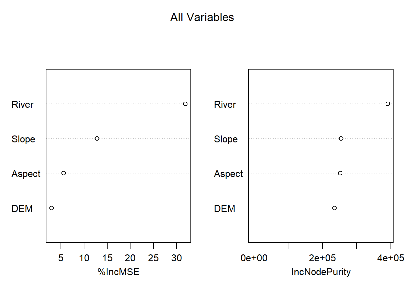
partialPlot(MeuseRF, Training.DF, River, , main = "PPD River")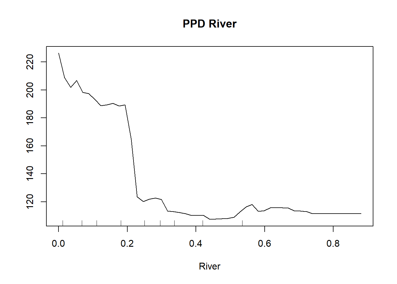
partialPlot(MeuseRF, Training.DF, Slope, , main = "PPD Slope")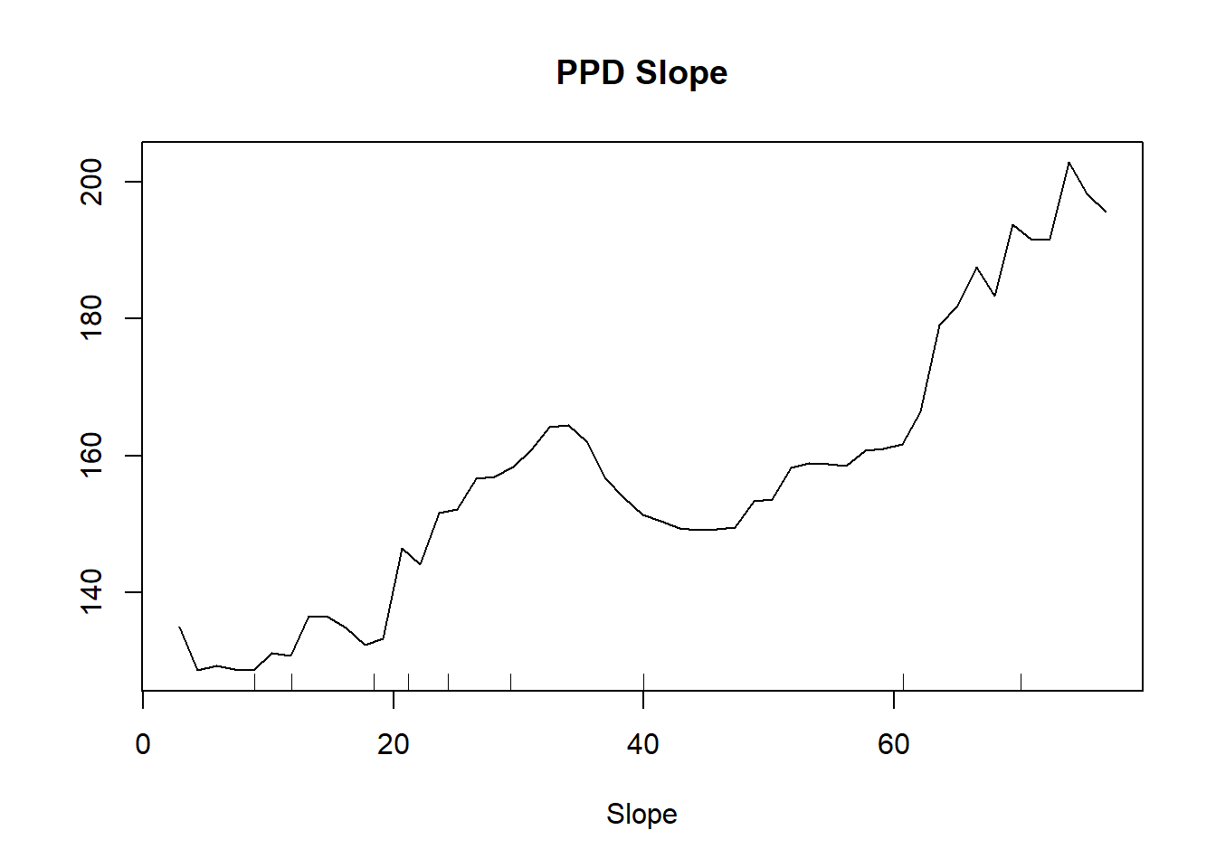
partialPlot(MeuseRF, Training.DF, DEM, , main = "PPD Elevation")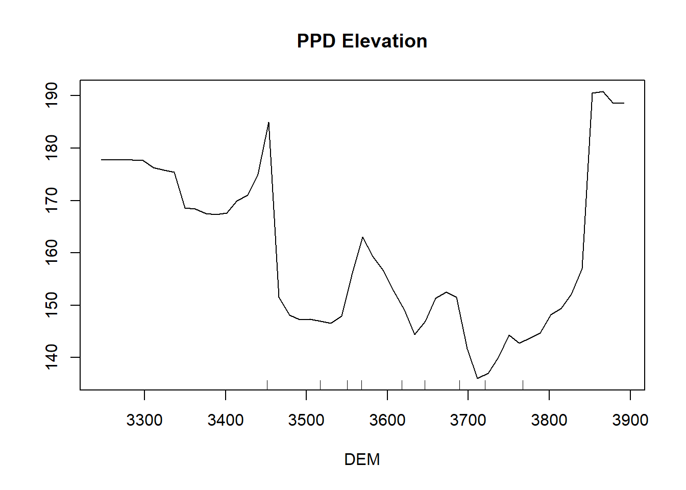
#to predict the RF to an output, we have to create a raster stack of our data so that it cant determine the optimal placement of valuesPredicting the output
to predict the RF to an output, we have to create a raster stack of our data so that it can determine the optimal placement of values
#Creating the Raster Stack
Stack.Meuse <-stack(DEM,Slope,Aspect,River)

#The names of the Raster Stack and the Training Dataframe were not lining up
names(Stack.Meuse) <- c("DEM","Slope","Aspect","River")

Lead <- predict(Stack.Meuse, MeuseRF, filename = "lead.tif", fun = predict, se.fit=TRUE, overwrite=TRUE)
## Warning in showSRID(uprojargs, format = "PROJ", multiline = "NO", prefer_proj
## = prefer_proj): Discarded datum Unknown based on Bessel 1841 ellipsoid in Proj4
## definitionplot(Lead, main= "Lead for the Meuse Data")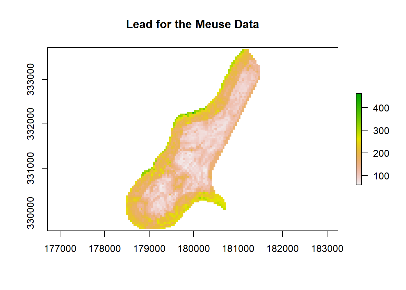
Christopher Scarpone, PhD, P.Ag.
I am an environmental scientist and Professional Agrologist (P.Ag.) focused on representing forests and landscapes in digital form, with an emphasis on LiDAR, urban forestry, and scalable analytical tools.